Problem
Given a graph which represents a flow network where every edge has a capacity. Also given two vertices source S and sink T in the graph. Find out the maximum possible flow from S to T with following constraints
- Flow on an edge doesn’t exceed the given capacity of the edge
- In-flow is equal to Out-flow for every vertex except s and t
Ford-Fulkerson Algorithm
The following is a simple idea of the algorithm
- Start with a initial maxFlow as 0
- While there is an augmenting path from source to sink Add this path flow to maxFlow
- Return maxFlow
Terminologies
- Residual Graph: It’s a graph which indicates additional possible flow. If there is such path from source to sink then there is a possibility to add flow
- Residual Capacity: It’s original capacity of the edge minus flow
- Minimal Cut: Also known as bottleneck capacity, which decides maximum possible flow from source to sink through an augmented path
- Augmenting path: Augmenting path can be done in two ways:
- Non-full forward edges
- Non-empty backward edges
**Not so clear, especially the 2nd one “Non-empty backward edges” :(, but we will get into it later in our example.
What Happens If Naive Algorithm is Applied
Lets assume we have simple graph with four vertices and five edges:
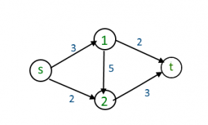
When the Naive Greedy Algorithm (GA) approach is applied the maximum flow may be not produced. It is well known from the definition of the greedy algorithm that every step it tries to grab maximum value. Which is not always brings to the collective maxmum solution.
- From the source GA chooses 3 because it has highest value
- From vertex 1 the GA would choose edge with value 5
- Finally from vertex 2 the GA chooses only left edge which is 3
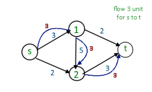
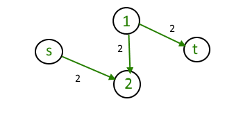 The GA ends the with the maximum flow 3, but actually the maximum flow 5 could be reached.
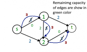
Residual Graphs
The main novelty idea behind the Residual Graph is that algorithm allows “undo” operations. When we flow back on the edge (means go agains the direction of the arrow) then we add the flow number to the edge value. Main constraints here is that adding up number should not be bigger than original flow value of the edge.
Step By Step Run
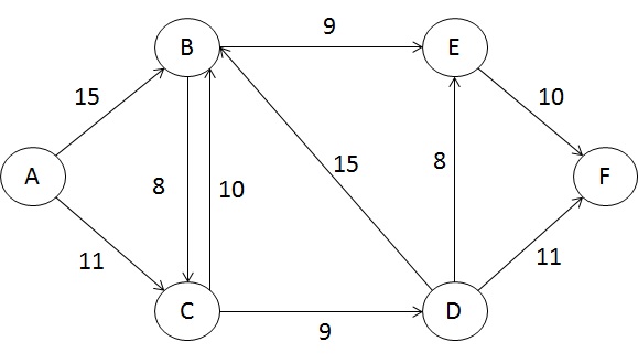
We are given the following graph:
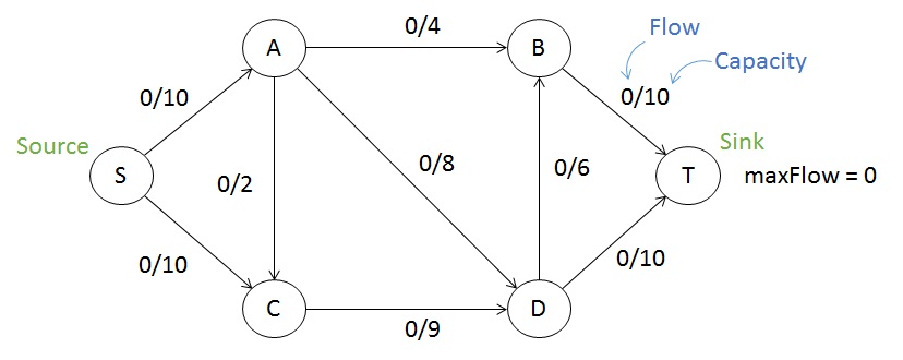
Here, S is source and T is the sink which is target destination. Our goal is to calculate the maximum flow for this graph
Lets, just consider a path S -> A -> D -> T
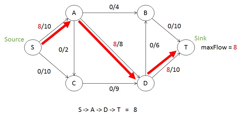
The chosen path is called augmentation path, and each edge has different capacity. For example S -> A has capacity 10, A -> D has capacity 8, D -> T has capacity 10. The edge A->D with capacity 8 is the smallest among other edges. That is why it is called minimal cut, more traditionally we call it a bottleneck. Now every edge subtracts the bottleneck (in this case 8) from its capacity. That is why we can write the subtracted 8 on the right side of the slash. As a result for S->A we have “8/10”, which means now this edge has capacity 2. Maximum Flow is the summation of the all “minimum cuts” at every step. We will get back to maximum flow later again.
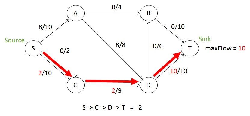
Lets, continue in a same fashion, this time we go by lower edge S->C edge
Now we chose the path S->C->D and when we reach D there is no direct way to the target, because the edge D->T is already full and has 0 capacity remained. The maximum flow definition has mentioned above “Non-empty backward edges”, which allow us to flow backward against the arrow. That is why D->A path can be used, as shown here:
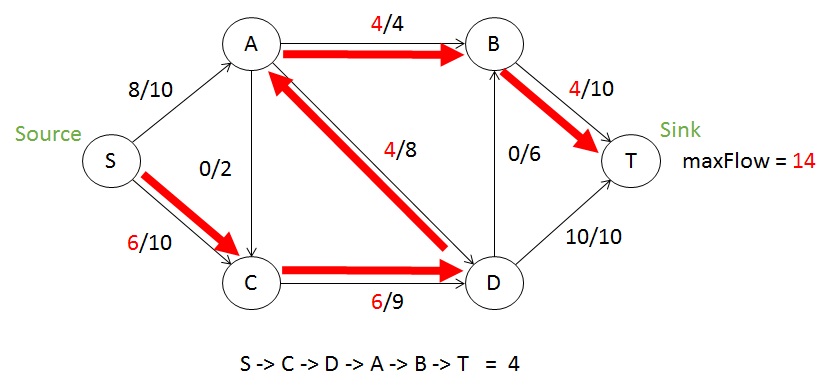
Let’s dive into details, and analyse whats happened here. The edge A->D already been full 8/8 (means 0 capacity left). But when we flow backward D->A we take away used flow that is why it becomes 4/8. In another word, we are adding the capacity to the edge. Yeah it sounds little confusing, but stay tuned. When we flow back and the minimum cut (bottleneck) for this step has been selected as 4 (because of A->B bottleneck), that is why now the edge A->D has capacity 4. It is kind of cancels out previous usage of the A->D capacity. Even though it sounds strange, mathematically it is absolutely correct and I think this is the key point of the whole Maximum Flow algorithm.
**Important to remember that it is possible to flow back on the edge only if it has been flewed forward before. The value for flowing back cannot be bigger than the already used capacity. Which means if the A->D has not been used in previous steps and still had full capacity then we could not flow back from D->A
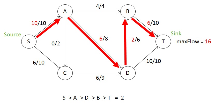
Now, we can continue the algorithm
and finally:
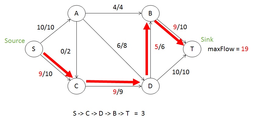
Now there is now way for flowing from S->T by augmenting any path. That is why we the algorithm stops here. Now we can list out all the augmented paths and bottleneck capacities on that step:
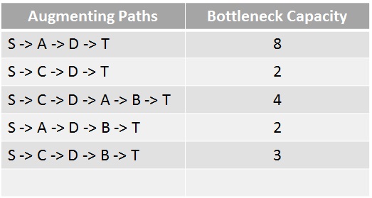
Summation of the bottleneck capacities for each step gives us the maximum flow result for this graph and it is 19.
Implementation
There are different implementations of the Ford Fulkerson Algorithm. The Edmonds-Karp Algorithm is the implementation of the Ford Fulkerson algorithm where the BFS is used for traversing through Graph. When the BFS is used the complexity can be reduced to O(VE^2)
Application Fields
- Data mining
- Open-pit mining
- Bipartite matching
- Network reliability
- Baseball elimination
- Image segmentation
- Network connectivity
- Distributed computing
- Egalitarian stable matching
- Security of statistical data
- Multi-camera scene reconstruction
- Sensor placement for homeland security
Bipartite Matching
There are dozens of real world problems that can be formed as Bipartite Matching. One of the popularly used one is Applicants and Jobs (mentioned by Robert Sedgewick in his Coursera MOOC):
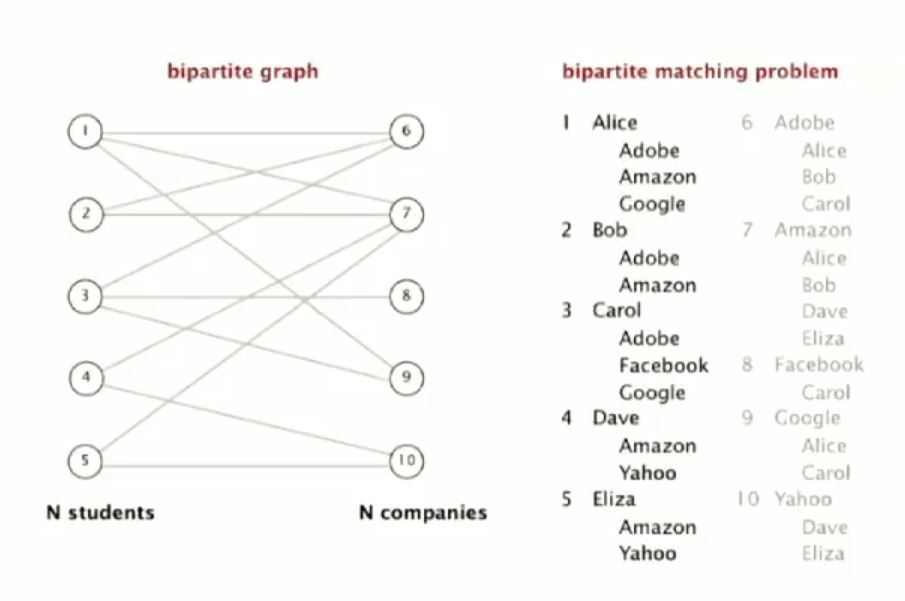
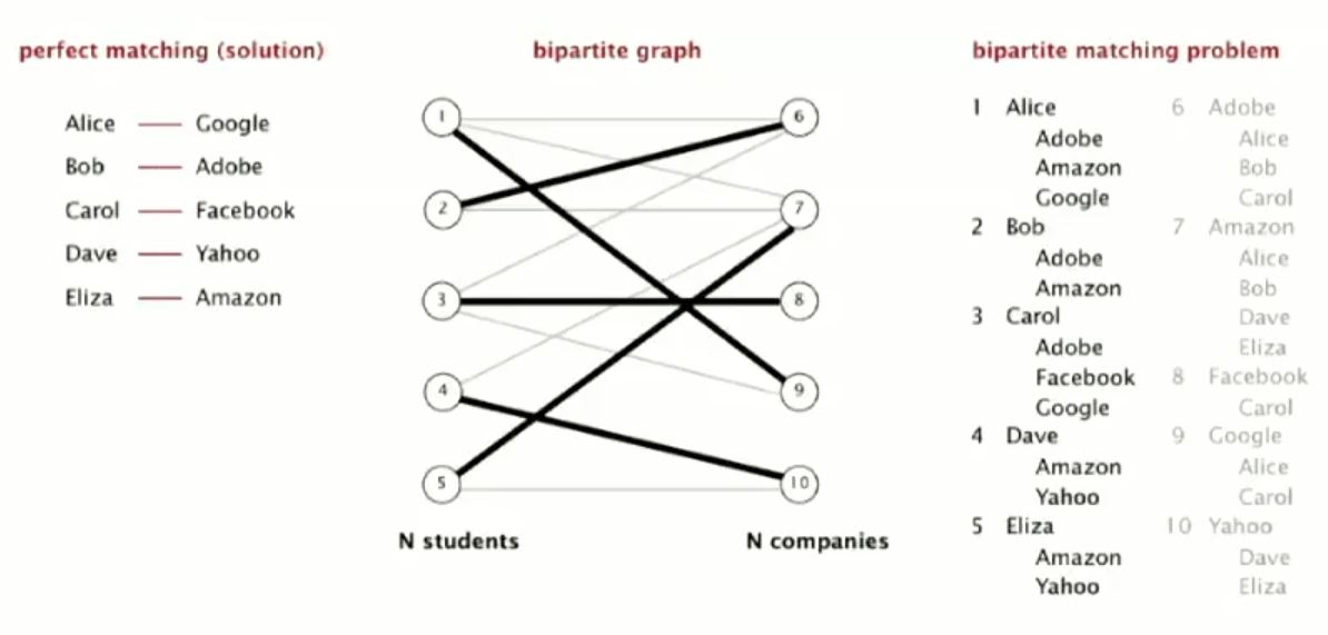
Alice has been accepted by Adobe, Amazon and Google. Bob has been accepted by Adobe and Amazon, and so on. Each of these jobs only receives one person. How should we perform matching that each of these applicants gets the job. This problem can be converted into maximum flow problem, and it has following solution:
Lets design it in the graph, using VisualAlgo web site, which I found really good tool for quick check:
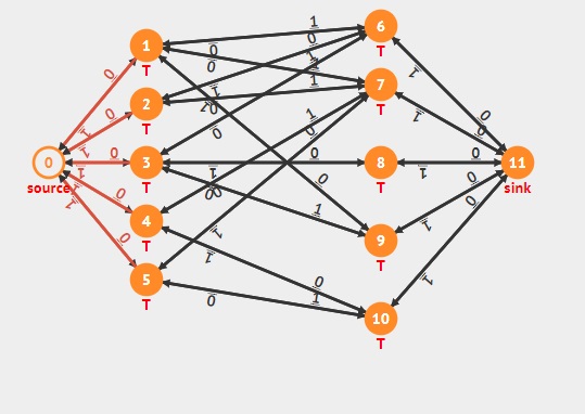
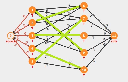
After designing the graph using VisualAlgo we can quick-run the algorithm for the result or check the solution step-by-step where each path augmentations are illustrated. Here the final solution and it perfectly matches with Robert Sedgwicks solution.
Try to Apply to Web Services
I have been looking around for different kinds of application examples, especially try to find web services related application. Couldn’t find one and decided to make my own.
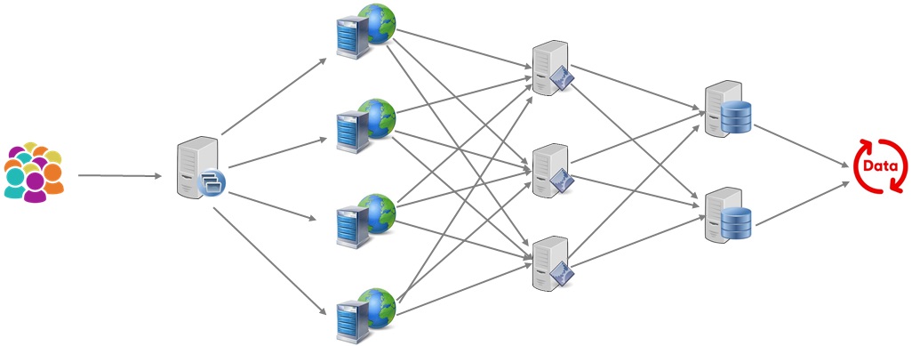
Here typical web architecture, with (right to left order) users, load balancer, web servers, application servers, databases and data itself. Two ends should be considered in an abstract way.
To make it look more examplistic (note sure such a word exist), lets give the weight to each edge, relative to the maximum load of the each server can handle. We are considering heterogeneous network and nodes.
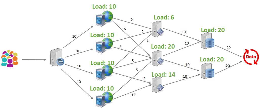
Now everything looks settled and ready to design the maximum flow. The goal of using maximum flow algorithm is to calculate what is the capability of this system and where are the bottlenecks.
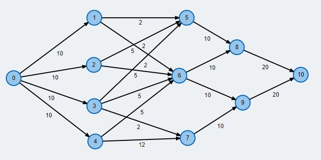
We have designed our network using another good online tool. Here you can see the source code of the model:
% Graph saved at Fri Sep 07 2018 22:43:41 GMT+0900 (Korean Standard Time)
n 25.267009493670884 203.61802184466018
n 206.91257911392407 352.88986650485435
n 205.80498417721518 236.38501213592232
n 206.91257911392407 134.4432645631068
n 209.1277689873418 47.064623786407765
n 415.1404272151899 352.88986650485435
n 398.52650316455697 209.68598300970874
n 417.35561708860763 55.55976941747573
n 528.1151107594936 280.0743325242718
n 541.40625 142.93841019417474
n 672.1024525316456 212.11316747572815
e 0 1 10
e 0 2 10
e 0 3 10
e 0 4 10
e 1 5 2
e 1 6 5
e 2 5 2
e 2 6 5
e 3 5 2
e 3 6 5
e 3 7 2
e 4 6 5
e 4 7 12
e 5 8 10
e 6 8 10
e 6 9 10
e 7 9 10
e 8 10 20
e 9 10 20
Lets, run the simulation and find out the maximum flow.
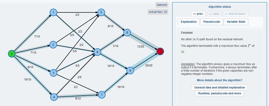
Here, we can see the maximum flow is equal to 33. Which is not something what we have expected. At the input we have 40 users connected, and on the right side we have the database with capability to serve 40 users. But somehow we are ending up serving only 33 users.
By applying maximum flow algorithms we can analyze and find bottlnecks of our systems.
Source Code
// Java program for implementation of Ford Fulkerson algorithm
import java.util.*;
import java.lang.*;
import java.io.*;
import java.util.LinkedList;

class MaxFlow
{
    static final int V = 6;    //Number of vertices in graph

    /* Returns true if there is a path from source 's' to sink
      't' in residual graph. Also fills parent[] to store the
      path */
    boolean bfs(int rGraph[][], int s, int t, int parent[])
    {
        // Create a visited array and mark all vertices as not
        // visited
        boolean visited[] = new boolean[V];
        for(int i=0; i<V; ++i)
            visited[i]=false;

        // Create a queue, enqueue source vertex and mark
        // source vertex as visited
        LinkedList<Integer> queue = new LinkedList<Integer>();
        queue.add(s);
        visited[s] = true;
        parent[s]=-1;

        // Standard BFS Loop
        while (queue.size()!=0)
        {
            int u = queue.poll();

            for (int v=0; v<V; v++)
            {
                if (visited[v]==false && rGraph[u][v] > 0)
                {
                    queue.add(v);
                    parent[v] = u;
                    visited[v] = true;
                }
            }
        }

        // If we reached sink in BFS starting from source, then
        // return true, else false
        return (visited[t] == true);
    }

    // Returns tne maximum flow from s to t in the given graph
    int fordFulkerson(int graph[][], int s, int t)
    {
        int u, v;

        // Create a residual graph and fill the residual graph
        // with given capacities in the original graph as
        // residual capacities in residual graph

        // Residual graph where rGraph[i][j] indicates
        // residual capacity of edge from i to j (if there
        // is an edge. If rGraph[i][j] is 0, then there is
        // not)
        int rGraph[][] = new int[V][V];

        for (u = 0; u < V; u++)
            for (v = 0; v < V; v++)
                rGraph[u][v] = graph[u][v];

        // This array is filled by BFS and to store path
        int parent[] = new int[V];

        int max_flow = 0;  // There is no flow initially

        // Augment the flow while tere is path from source
        // to sink
        while (bfs(rGraph, s, t, parent))
        {
            // Find minimum residual capacity of the edhes
            // along the path filled by BFS. Or we can say
            // find the maximum flow through the path found.
            int path_flow = Integer.MAX_VALUE;
            for (v=t; v!=s; v=parent[v])
            {
                u = parent[v];
                path_flow = Math.min(path_flow, rGraph[u][v]);
            }

            // update residual capacities of the edges and
            // reverse edges along the path
            for (v=t; v != s; v=parent[v])
            {
                u = parent[v];
                rGraph[u][v] -= path_flow;
                rGraph[v][u] += path_flow;
            }

            // Add path flow to overall flow
            max_flow += path_flow;
        }

        // Return the overall flow
        return max_flow;
    }

    // Driver program to test above functions
    public static void main (String[] args) throws java.lang.Exception
    {
        // Let us create a graph shown in the above example
        int graph[][] =new int[][] { {0, 16, 13, 0, 0, 0},
                                     {0, 0, 10, 12, 0, 0},
                                     {0, 4, 0, 0, 14, 0},
                                     {0, 0, 9, 0, 0, 20},
                                     {0, 0, 0, 7, 0, 4},
                                     {0, 0, 0, 0, 0, 0}
                                   };
        MaxFlow m = new MaxFlow();

        System.out.println("The maximum possible flow is " +
                           m.fordFulkerson(graph, 0, 5));

    }
}
References
- Good Visual site for checking how the max-flow works: https://visualgo.net/en/maxflow
- Another good maximum flow calculator made by some German student https://www-m9.ma.tum.de/graph-algorithms/flow-ford-fulkerson/index_en.html