Usually, the sorting algorithms determine the sort based on comparisons between the input elements. That is why they called comparison sorts algorithms. In here we would like to consider non-comparison sorts.
Counting sort
Counting sort assumes that each of the n input elements is an integer in the range 0 to k, for some integer k. When k=O(n), the sort runs in O(n) time
Counting sort works based on counting frequency of each element, by counting them.
COUNTING-SORT(A, B, k):
let C[0..k] be a new array
for i = 0 to k
   C[i] = 0
for j = 1 to A.length
   C[A[j]] = C[A[j]] + 1
// C[i] now contains the number of elements equal to i
for i = 1 to k
   C[i] = C[i] + C[i - 1]
// C[i] now contains the number of elements less than or equal to i
for j = A.length downto 1
   B[C[A[j]]] = A[j]
   C[A[j]] = C[A[j]] - 1
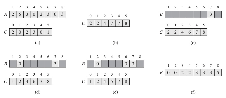
Array C is used to collect the frequency of each element. Then the magical for loop does the main job:
for i = 1 to k
   C[i] = C[i] + C[i - 1]
This magic loop conversts frequency array C = [2,0,2,3,0,1] into C = [2,2,4,7,7,8] array who holds the information about how many less and equal elements are exists from current index. It all becomes clear when we reach the final loop
for j = A.length downto 1
   B[C[A[j]]] = A[j]
   C[A[j]] = C[A[j]] - 1
As we can see now C array holds the position of the elements from array A. Notice: I’m not sure but do we really have to go backward in a final loop? Because it seems to me, it could work even if we just go from 1 to A.length
Radix sort
The idea of Radix Sort is to do digit by digit sort starting from least significant digit to most significant digit. Radix sort uses counting sort as a subroutine to sort.
RADIX-SORT(A, d)
for i = 1 to d
    use a stable sort to sort array A on digit i
Here another good example from geeksforgeeks:
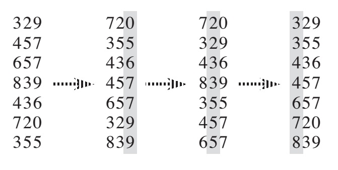
Original, unsorted list:

170, 45, 75, 90, 802, 24, 2, 66
Sorting by least significant digit (1s place) gives: [*Notice that we keep 802 before 2, because 802 occurred before 2 in the original list, and similarly for pairs 170 & 90 and 45 & 75.]

170, 90, 802, 2, 24, 45, 75, 66
Sorting by next digit (10s place) gives: [*Notice that 802 again comes before 2 as 802 comes before 2 in the previous list.]


802, 2, 24, 45, 66, 170, 75, 90
Sorting by most significant digit (100s place) gives:

2, 24, 45, 66, 75, 90, 170, 802
When each digit is in the range 0 to k-1 (so that it can take on k possible values), and k is not too large, counting sort is the obvious choice.
Bucket Sort
Bucket sort assumes that the input is drawn from a uniform distribution and has an average-case running time of O(n). Like counting sort, bucket sort is fast because it assumes something about the input.
BUCKET-SORT(A):
let B[0..n-1] be a new array
n = A.length
for i = 0 to n - 1
   make B[i] an empty list
for i = 1 to n
   insert A[i] into list B[floor(n * A[i])]
for i = 0 to n - 1
   sort list B[i] with insertion sort
concatenate the list B[0], B[1], ..., B[n-1] together in order
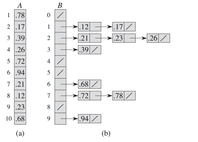
Detail calculations:
0.72 * 10 = 7.2 -> ceil() -> 7
0.17 * 10 = 1.7 -> ceil() -> 1
...
...
0.68 * 10 = 6.8 -> ceil() -> 6
To analyze the cost of the calls to insertion sort, let n[i] be the random variable denoting the number of elements placed in bucket B[i]. Since insertion sort runs in quadratic time. As conclusion the average-case running time for bucket sort is:
O(n) + n * O(2 - 1/n) = O(n)
Even if the input is not drawn from a uniform distribution, bucket sort may still run in linear time. As long as the input has the property that the sum of the sum squares of the bucket sizes is linear in the total number of elements.
The disadvantage is that if you get a bad distribution into the buckets, you may end up doing a huge amount of extra work for no benefit or a minimal benefit. As a result, bucket sort works best when the data are more or less uniformly distributed or where there is an intelligent way to choose the buckets given a quick set of heuristics based on the input array